How to use replicate weights with SAS - American Community Survey or Current Population SurveyFor some reason, there are negative replicate weights in the ACS data. (I don’t know if this is the case with the CPS data.) data acs; set a.acs; array temp(*) pwgtp1-pwgtp80; do i = 1 to dim(temp); if temp(i) < 0 then temp(i)=0; end; run; proc surveymeans data = indiana varmethod=jackknife; var agep; weight pwgtp; repweights pwgtp1-pwgtp80 / jkcoefs=0.05; run; The value for jkcoefs (4/80=0.05) comes from the documentation for variance estimation (chapter 12 of the design methodology):

For some reason, there are negative replicate weights in the ACS data. (I don’t know if this is the case with the CPS data.) See also IPUMS.

data acs;
 set a.acs;
 array temp(*) pwgtp1-pwgtp80;

 do i = 1 to dim(temp);
   if temp(i) < 0 then temp(i)=0;
 end;
run;

proc surveymeans data = indiana varmethod=jackknife;
var agep;
weight pwgtp;
repweights pwgtp1-pwgtp80 / jkcoefs=0.05;
run;

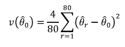
The value for jkcoefs (4/80=0.05) comes from the documentation for variance estimation (chapter 12 of the design methodology):

Update: I believe the following statements will also work but haven't verified this:

proc surveymeans data = indiana varmethod=brr (fay=0.5);
var agep;
weight pwgtp;
repweights pwgtp1-pwgtp80;
run;

Convert pre-2002 CPS industry and occupation codes

The idea is straightforward. Most of the pre-2002 occupations have been redistributed into other occupations post-2002. In order to get to the new codes generate a random number over the entire data set. If the old occupation has a random number within the range defined by Census then we set this to be its new code.

The rules for the proportions of old occupations and industries to be redistributed to the new codes are available at the Census web site or at IPUMS. The spreadsheets containing the rules for industry were downloaded from here while the rules for the occupations were downloaded from here.

The caveats are that the porportions are assumed to remain constant over time and that the data set is large enough that how the random numbers are generated does not matter 'much'.

The SAS code first converts the occupation spreadsheet to SAS data to be written out to a text file:

PROC IMPORT OUT= WORK.temp 
            DATAFILE= "I:\occ_90-00.xls" 
            DBMS=EXCEL REPLACE;
     RANGE="Sheet1$"; 
     GETNAMES=YES;
     MIXED=YES;
     SCANTEXT=YES;
     USEDATE=YES;
     SCANTIME=YES;
RUN;

data temp1(drop = Table_2___1990_Census_Occupation f6);
  set temp(drop = f5 f7 f8);
  rename /* Table_2___1990_Census_Occupation = oldcode*/
    f2 = oldlabel f3 = newcode f4 = newlabel ;
  if _N_ < 5 then delete; 
  if index (Table_2___1990_Census_Occupation, 'categor')>0 then delete;
  oldcode = input (Table_2___1990_Census_Occupation,4.);
  if f6 ne 'NA' then percent = input(f6, 8.);
run;

data temp1(drop = oldcode oldlabel newcode);
  retain c clabel;
  length clabel $ 65;
  set temp1;
  if oldcode ne . then c = oldcode;
  if oldlabel ne ' ' then clabel = oldlabel;
  ncode = input(newcode, 4.);
  if percent = . then delete;
run;

data temp2;
  retain c ncode;
  set temp1(where = (ncode ne .)); by c;
  retain cumpct;
  if first.c then do; 
    cumpct = percent;
    lpercent = 0;
  end;
  else do;
    lpercent = cumpct;
    cumpct = cumpct + percent;
  end;
run;

data _null_;
  set temp2; by c;
  file "I:\CPS\SAS Programs\occ1990_2000_xwalk.sas";
  if first.c then do;
    if _N_ = 1 then put "if old_code = " c " then do;";
    else put "else if old_code = " c " then do;";
    put "  if " lpercent "< y <= " cumpct " then new_code = " ncode ";";
  end;
  else if not first.c then do;
    put "  if " lpercent "< y <= " cumpct " then new_code = " ncode ";";
  end;
  if last.c then do;
  put "end;";
  end;
run;

The following does the same for industry:

PROC IMPORT OUT= WORK.temp 
            DATAFILE= "I:\ind_90-00.xls" 
            DBMS=EXCEL REPLACE;
     RANGE="Sheet1$"; 
     GETNAMES=YES;
     MIXED=NO;
     SCANTEXT=YES;
     USEDATE=YES;
     SCANTIME=YES;
RUN;

data temp1;
  set temp(drop = f5 f7 f8);
  rename Table_1___1990_Census_Industry_C = oldcode
    f2 = oldlabel f3 = newcode f4 = newlabel f6 = percent;
  if _N_ < 5 then delete; 
  if index (Table_1___1990_Census_Industry_C, 'categor')>0 then delete;
run;

data temp1(drop = oldcode oldlabel newcode);
  retain c clabel;
  length clabel $ 65;
  set temp1;
  if oldcode ne ' ' then c = input(oldcode, 4.);
  if oldlabel ne ' ' then clabel = oldlabel;
  ncode = input(newcode, 4.);
  if percent = . then delete;
run;

data temp2;
  retain c ncode;
  set temp1; by c;
  retain cumpct;
  if first.c then do; 
    cumpct = percent;
    lpercent = 0;
  end;
  else do;
    lpercent = cumpct;
    cumpct = cumpct + percent;
  end;
run;

data _null_;
  set temp2; by c;
  file "I:\CPS\SAS Programs\ind1990_2000_xwalk.sas";
  if first.c then do;
    if _N_ = 1 then put "if old_code = " c " then do;";
    else put "else if old_code = " c " then do;";
    put "  if " lpercent "< x <= " cumpct " then new_code = " ncode ";";
  end;
  else if not first.c then do;
    put "  if " lpercent "< x <= " cumpct " then new_code = " ncode ";";
  end;
  if last.c then do;
  put "end;";
  end;
run;

Now there are two SAS programs to be included. First a search and replace is used to replace the "old_code" to PEIO1OCD (occupation) and PEIO1ICD (industry) and "new_code" to NEW_OCC and NEW_IND respectively (for example). It would have been simpler to have SAS write them out but I wanted to be able to use this if some other data set used a different variable name and I needed to remember which was old and new. The following is a snippet to do the actual recode:

  call streaminit (6875309&yr);
  x  = rand('uniform') * 100;
  y  = rand('uniform') * 100;
  
  %include "occ1990_2000_xwalk.sas";
  %include "ind1990_2000_xwalk.sas";

Here's a snippet of what the actual code will look like (for occupation):

if peio1ocd = 3  then do;
  if 0 < y <= 100  then peio1ocd_r = 3 ;
end;
else if peio1ocd = 4  then do;
  if 0 < y <= 77.143  then peio1ocd_r = 1 ;
  if 77.143 < y <= 100  then peio1ocd_r = 43 ;
end;
else if peio1ocd = 5  then do;
  if 0 < y <= 1.571  then peio1ocd_r = 1 ;
  if 1.571 < y <= 4.712  then peio1ocd_r = 2 ;
  if 4.712 < y <= 6.806  then peio1ocd_r = 10 ;
  if 6.806 < y <= 8.377  then peio1ocd_r = 11 ;
  if 8.377 < y <= 13.613  then peio1ocd_r = 12 ;
  if 13.613 < y <= 14.66  then peio1ocd_r = 13 ;
  if 14.66 < y <= 16.754  then peio1ocd_r = 15 ;
  if 16.754 < y <= 17.278  then peio1ocd_r = 16 ;
  if 17.278 < y <= 17.802  then peio1ocd_r = 22 ;
  if 17.802 < y <= 19.896  then peio1ocd_r = 23 ;
  if 19.896 < y <= 20.42  then peio1ocd_r = 30 ;
  if 20.42 < y <= 20.944  then peio1ocd_r = 36 ;
  if 20.944 < y <= 21.991  then peio1ocd_r = 41 ;
  if 21.991 < y <= 26.703  then peio1ocd_r = 42 ;
  if 26.703 < y <= 67.541  then peio1ocd_r = 43 ;
  if 67.541 < y <= 71.73  then peio1ocd_r = 54 ;
  if 71.73 < y <= 73.824  then peio1ocd_r = 62 ;
  if 73.824 < y <= 76.965  then peio1ocd_r = 81 ;
  if 76.965 < y <= 77.489  then peio1ocd_r = 84 ;
  if 77.489 < y <= 82.725  then peio1ocd_r = 93 ;
  if 82.725 < y <= 88.484  then peio1ocd_r = 122 ;
  if 88.484 < y <= 89.008  then peio1ocd_r = 164 ;
  if 89.008 < y <= 91.102  then peio1ocd_r = 202 ;
  if 91.102 < y <= 93.72  then peio1ocd_r = 211 ;
  if 93.72 < y <= 94.244  then peio1ocd_r = 215 ;
  if 94.244 < y <= 94.768  then peio1ocd_r = 354 ;
  if 94.768 < y <= 95.292  then peio1ocd_r = 382 ;
  if 95.292 < y <= 95.816  then peio1ocd_r = 395 ;
  if 95.816 < y <= 100.005  then peio1ocd_r = 525 ;
end;

SAS Graphics

Doing graphs in SAS is a pain – mainly because of the fact that options for high resolution graphics are device specific. JPEG is what I usually work with for inclusion into LaTex documents but they never come out as crisp as I like them to be. What the SAS folks really need to do is come out with specific recommendations for specific types of output: JPEG, BMP, etc for specific types of purposes, that is if we want to use this type of image for a journal article, what should the options be. What if I want to use them for a web page? What are the options for a 3x5 or a 4x6?

I realize that the combinations can be mind boggling but they really need to lay down some kind of recommendations because I ended up spending two hours trying to get the graphics options just right for a high resolution JPEG for 3x5 in.

This was what I came up with for Windows 7, SAS 9.2 Release 1:

goptions reset=all gsfmode=replace device = jpeg gsfname = grafout htext=0.9 fontres=presentation ftext=Verdana xmax=6in ymax=6in hsize=5in vsize=3.5in xpixels=3600 ypixels=3600;

Unfortunately, even with running PROC FONTREG I keep getting the message that font 'Verdana' cannot be used. Oh well, I'll have to figure it out another day when I have two hours to kill.

Finding the most common element in an array using SAS

Found a need for this a while back - nothing fancy here - if there is a tie only the first most commonly occuring element is listed.

/* Create a data set of 1000 records. An array of 10 elements is also created - we want to find the most commonly occuring element */
data temp;
  array a(*) a1 - a10;

  do id = 1 to 1000;
     do j = 1 to 10;
     call streaminit(215582 + id * j);
     a(j) = round(rand('normal',5,4)) ;
   end;
   output;
  end;
  drop j;
run;

data temp;
  set temp;
  
  array a(*) a1-a10;
  call sortn(of a(*));
  count = 0; mode_count = 0;
  do i = 1 to dim(a)-1;
    if a(i) = a(i+1) and a(i) ne . and a(i+1) ne . then do;
    find_first = a(i);
    count = count + 1;
  end;
  else if a(i) ^= a(i+1) and a(i) ne . and a(i+1) ne . then do;
    if count > mode_count then do;
      mode = find_first;
      mode_count = count;
    end;
    count = 0;
  end;
  end;
  /* The last elements are the most frequently occuring once we reach the end of the array and a mode has not yet been found */
  if mode = . and count > 1 then do;
    mode = a(dim(a)); 
  mode_count = count;
  end;
  /* If we reach the end of the array and count is greater than mode count then this must also be the most frequently occuring */
  if count > mode_count then do;
    mode = a(dim(a)); 
  mode_count = count;
  end;
  drop i;
run;

/* Now let's check if it finds the correct ones */
proc transpose data = temp out=ttemp prefix=id;
id id;
var a1-a10;
run;

proc means data = ttemp mode noprint;
var id1-id1000;
output out = checkmode(drop = _type_ _freq_) mode=cmode1-cmode1000;
run;

proc transpose data = checkmode out = c prefix=checkmode;
var cmode1-cmode1000;
run;

data c;
  set c(drop = _name_);
  id = _N_;
run;

data ctemp;
  merge temp c; by id;
  if checkmode1 ne mode then flag = 1;
run;

data wrong(drop = find_first flag);
  set ctemp;
  where flag = 1;
run;

/* In macro form */
%macro array_mode(arrayname=);
  call sortn(of &arrayname(*));
  count = 0; mode_count = 0;
  do i = 1 to dim(&arrayname)-1;
    if &arrayname(i) = &arrayname(i+1) and &arrayname(i) ne . and &arrayname(i+1) ne . then do;
    find_first = &arrayname(i);
    count = count + 1;
  end;
  else if &arrayname(i) ^= &arrayname(i+1) and &arrayname(i) ne . and &arrayname(i+1) ne . then do;
    if count > mode_count then do;
      mode = find_first;
      mode_count = count;
    end;
    count = 0;
  end;
  end;
  /* The last elements are the most frequently occuring once we reach the end of the array and a mode has not yet been found */
  if mode = . and count > 1 then do;
    mode = &arrayname(dim(&arrayname)); 
  mode_count = count;
  end;
  /* If we reach the end of the array and count is greater than mode count then this must also be the most frequently occuring */
  if count > mode_count then do;
    mode = &arrayname(dim(&arrayname)); 
  mode_count = count;
  end;
  drop i;
%mend array_mode;

Replicating Econbrowser's replication of CEA analysis

There was an interesting post on Econbrowser where the impact of the fiscal stimulus done by the CEA was replicated.

options nocenter;
filename gdp 'C:\ReplicateCEA\GDPC1.txt';
/* File downloaded from FRED St. Louis */
data GDP;
infile gdp firstobs = 14;
/* Read two variables: date and GDP */
input date value;
informat date yymmdd10.;
format date yymmdd10.;
lngdp = log(value);
y=lngdp;
/* Calculate the first difference of y */
diffy = dif(y);
run;

data gdp4q;
set GDP end=last;
output;
if last then do;
date = '01Oct2009'd;
value = value * 1.04;
lngdp = log(value);
y=lngdp;
output;
end;
run;

data gdp4q;
set gdp4q;
dateq = put(date,yyq6.);
run;

filename nfp 'C:SVAR\ReplicateCEA\PAYEMS.txt';
/* File downloaded from FRED St. Louis */
data NFP;
infile nfp firstobs = 16;
/* Read two variables: date and GDP */
input date value;
informat date yymmdd10.;
format date yymmdd10.;
lnnfp = log(value);
e=lnnfp;
/* Calculate the first difference of y */
diffnfp = dif(e);
dateq = put(date,yyq6.);
run;

data nfp2;
set nfp; by dateq date;

if last.dateq then output;
run;

data gdp_nfp(drop = ln: diff:);
merge gdp4q(in=a rename = (value = gdp)) nfp2(in=b rename = (value = nfp));

by dateq;
if a and b;
run;

proc print data = gdp_nfp noobs;
where year(date)>=2007;
run;

ods output ParameterEstimates=pe;
proc varmax data = gdp_nfp;
where 1990<=year(date)<=2007;
id date interval = qtr;
model y e /p=4 ;
output lead=12 out = for;
run;

proc transpose data = pe out = pe_ty;
where equation = 'y';
var estimate;
id parameter;
run;

data pe_ty;
set pe_ty(rename = (const1 = intercept) drop = _name_);
_type_ = 'PARMS';
_model_ = 'Baseline';
_depvar_ = 'y';
y = -1;
RUN;

proc transpose data = pe out = pe_te;
where equation = 'e';
var estimate;
id parameter;
run;

data pe_te;
set pe_te(rename = (const2 = intercept) drop = _name_);
_type_ = 'PARMS';
_model_ = 'Baseline';
_depvar_ = 'e';
e = -1;
RUN;

%macro genar(lag=,eq1=,eq2=,var1=,var2=);
%do i=1 %to &lag;
%do e=1 %to &eq2;
ar&i._&eq1._&e=lag&i(&&var&e);
%end;
%end;
%mend genar;

options mprint;
data gdp2;
set gdp_nfp;
%genar(lag=4,eq1=1,eq2=2,var1=y,var2=e);
run;

data e2;
set gdp_nfp;
%genar(lag=4,eq1=2,eq2=2,var1=y,var2=e);
run;

proc score data = gdp2 score = pe_ty out=gdp2_score type=parms;
var ar1_1_1 ar1_1_2 ar2_1_1 ar2_1_2 ar3_1_1 ar3_1_2 ar4_1_1 ar4_1_2;
run;

proc score data = e2 score = pe_te out=e2_score type=parms;
var ar1_2_1 ar1_2_2 ar2_2_1 ar2_2_2 ar3_2_1 ar3_2_2 ar4_2_1 ar4_2_2;
run;

symbol1 value=none i=join;
symbol2 value=none i=join;
proc gplot data = gdp2_Score;
where year(date)>=2008;
plot (baseline y) * date / overlay;
run;
quit;

proc gplot data = e2_score;
where year(date)>=2008;
plot (baseline e) * date / overlay;
run;
quit;

Average monthly condo fees in the U.S.

Data source:

Steven Ruggles, Matthew Sobek, Trent Alexander, Catherine A. Fitch, Ronald Goeken, Patricia Kelly Hall, Miriam King, and Chad Ronnander. Integrated Public Use Microdata Series: Version 4.0 [Machine-readable database]. Minneapolis, MN: Minnesota Population Center [producer and distributor], 2008.

We've been looking at condos around the DC area and it got me wondering as to what the average condo fees were like around the country. The above is a chart of the average condo fees tabulated from IPUMS. Because of topcoding the average is below the true average. The mean and max are labeled at the end of the bars. Unfortunately, I'm unable to improve on the resolution of the jpeg.

The SAS code for this is:

proc means data = cf.hh2008 N mean std min max;
where year = 2008 and condofee > 0;
class stateicp;
var condofee;
weight hhwt;
output out = summ mean = meancondofee min = mincondofee max=maxcondofee;
run;

data summ2;
set summ;
proc sort; by descending meancondofee;
run;

data annosum;
set summ2;
%annomac;
%dclanno;
%system(2,2,3);
midpoint = stateicp;
x = round(meancondofee,1);
lbl = compress(put(meancondofee, 8.)"/"put(maxcondofee, 8.));
%label(x,.,lbl,black,0,0,1.8,swissb,6);
run;

filename grafout 'chart1.jpeg';
goptions device = jpeg targetdevice = jpeg ftext="Verdana" gsfname = grafout xmax=8 in ymax=6 in xpixels=4000 ypixels=3000 vpos=40 hpos=40 lfactor=1 ;
axis1 label = none;
title1 h=1 'Average monthly condominium fees in 2008: U.S. States';
proc gchart data=summ2;
where _type_ ^=0;
hbar stateicp / sumvar=meancondofee maxis=axis1 discrete descending nostat anno=annosum(where=(_type_^=0));
run;
quit;

Generating correlated random variables using SAS

This code is based on the discussion on SITMO. It uses two ways to generate correlated random variables. For any correlation matrix, C,

1) Find the Cholesky decomposition. In SAS, this uses the root function in IML. Multiply the Cholesky decomposition to a matrix of randomly generated numbers.

2) Find the eigenvalues and eigenvectors. In SAS, the function is call eigen in IML. The eigenvectors pre-multiplied with the diagonalized eigenvalues results in a matrix V. Multiply the transpose of V with the matrix of randomly generated numbers.

The product of this multiplication results in a matrix of correlated series.

The code:

proc iml;
C={1 0.6 0.3, 0.6 1 0.5, 0.3 0.5 1};
/* Method 1 uses the Cholesky decomposition */
U=root(C);
/* Method 2 uses the eigenvalues and eigenvectors */
call eigen(eival, eivec, c);
v=eivec*(diag(sqrt(eival)));
vt=t(v);
call randseed(12345);
/* Generate 3 random series 500 in length */
randm = j(500,3,.);
call randgen(randm,'NORMAL');
corr = randm * U;
corrv = randm * vt;
create random_data from randm;
append from randm;
create correlated_data from corr;
append from corr;
create correlated_data_v from corrv;
append from corrv;
quit;

title1 'Correlation of randomly generated data';
proc corr data = random_data;
run;

title1 'Correlation of data using Cholesky decomposition';
proc corr data = correlated_data;
run;

title1 'Correlation of data using Eigenvalue and Eigenvector decomposition';
proc corr data = correlated_data_v;
run;

Note that the correlation using 500 numbers may not give the exact correlation as in the C matrix. A longer series may be required, e.g. 1000.

Overlaying/superimposing NBER recession dates on time series

I don't really know what you'd call it but I've always been curious how Econbrowser produces nice charts like this one on recession probabilities. I'm a SAS geek and this is how I coded it although I think that SAS should have an easier way of doing this without having to use an ANNOTATE data set which despite having used it quite a lot on project work is still a little bit of a mystery to me. Unfortunately, I don't know enough about HTML to render the code correctly so the input statement looks wrong.

data NBERdates;
   length PeakQ $ 20 TroughQ $ 20;
   informat Peak Trough ddmmyy10.;
   format Peak Trough date9.;
   input PeakQ 1-20 TroughQ 21-40 Peak Trough;
datalines;
February 1945(I)    October 1945 (IV)   1/2/1945        1/10/1945
November 1948(IV)   October 1949 (IV)   1/11/1948       1/10/1949
July 1953(II)       May 1954 (II)       1/7/1953        1/5/1954
August 1957(III)    April 1958 (II)     1/8/1957        1/4/1958
April 1960(II)      February 1961 (I)   1/4/1960        1/2/1961
December 1969(IV)   November 1970 (IV)  1/12/1969       1/11/1970
November 1973(IV)   March 1975 (I)      1/11/1973       1/3/1975
January 1980(I)     July 1980 (III)     1/1/1980        1/7/1980
July 1981(III)      November 1982 (IV)  1/7/1981        1/11/1982
July 1990(III)      March 1991(I)       1/7/1990        1/3/1991
March 2001(I)       November 2001 (IV)  1/3/2001        1/11/2001
;
run;

data NBERdates;
    set NBERdates;
    where Peak > '01Jan1947'd and Peak < '31Dec2000'd;
    PeakS = "'"put(Peak, date9.)"'d";
    TroughS = "'"put(Trough, date9.)"'d";
run;

filename gdp 'GDPC1.txt'; /* File downloaded from FRED St. Louis */
data GDP;
   infile gdp firstobs = 14;
   /* Read two variables: date and GDP */
   input date value;
   informat date yymmdd10.;
   format date yymmdd10.;
   lngdp = log(value);
   /* We will refer to Y instead of LNGDP for consistent notation */
   y=lngdp;
   /* Calculate the first difference of y */
   diffy = dif(y);
run;

%annomac;

data NBERDate1;
    set NBERdates;
    date = Peak; output;
    date = Trough; output;
run;

data anno;
    merge GDP(rename = (y=y1)) NBERdate1; by date;
    RETAIN YSYS XSYS '2';
    %bar(Peak,7.3,Trough,9.2,ligr,0,S);
run;

goptions ftext = swiss fontres = presentation htext = 0.9;
axis1 label = (angle=90);
axis2 order = ('1Jan1945'd to '30Jun2000'd by year5) minor = none;
symbol1 color = red interpol = j;
symbol2 color = black interpol = j;

proc gplot data = GDP;
plot lngdp * date /legend vaxis = axis1 haxis = axis2 annotate = anno chref=blue;
format date yyq6.;
run;
quit;